Six Numbers, One Decision: What Really Lies Behind Equivalent Stress

A solid steel cube sinks to 10 kilometres of ocean depth. Around 100 MPa presses on each of its faces. And its equivalent stress? Practically zero.

If that makes you pause, you're in the right place. This is exactly where the difference lies between the colour value you read off a contour plot and the understanding behind it.

Almost everyone who works with FEM eventually reads "von Mises" off a colourful plot. What's usually less clear is what that single number actually summarises, and why it can be zero when the part is clearly under load. This article works from the bottom up: from force per area, which anyone recognises from their first engineering-mechanics lecture, to the yield surface in stress space. And because you understand it better when you can turn the dials, you can reproduce every step yourself in the Stress Space Explorer embedded at the end of this article.

Start at the bottom: stress is force per area

σ = F / A. Force divided by area, in MPa (N/mm²). Same as pressure, just acting on a solid body.

An everyday image: the same person creates enormous stress in the floor on a stiletto heel and tiny stress on a flat shoe. Same force, different area.

At a hypothetical cut through the body, this force can act in two ways: perpendicular to the cut as normal stress σ (tension or compression), or parallel to it as shear stress τ (shearing off). A tug-of-war rope is normal stress; scissors cutting paper are shear. Both are present at every point simultaneously.

Why one number isn't enough

Here comes the first uncomfortable point. If you place a different hypothetical cut through the same point, you measure different values there. Rotate the cut, and normal and shear stresses change with it.

So one number doesn't describe the state at a point. You write out the stresses for three perpendicular directions (x, y, z) and get three normal stresses (σx, σy, σz) and three shear stresses (τxy, τyz, τxz). That is the stress tensor: six independent values that completely describe the state at exactly one point.

Six numbers, then. And now the problem.

Six values, one limit

Your material data sheet knows a single limit: the yield strength Re. It is measured in the uniaxial tensile test, where only one stress acts and all others are zero.

So on one side you have the full stress state with six values. On the other, a single number from a very simple experiment. How do you compare that fairly?

The answer is an equivalent stress σv: a rule that translates the full state into one number you can hold directly against Re. The real question is now just moved, not solved: which rule is the right one, and why exactly that one?

The core idea: not every stress does equal damage

Here comes the central idea. You split the stress state into two parts:

• Hydrostatic: the average of the three normal stresses, acting like uniform pressure or tension from all sides. It only changes the volume; the shape stays.
• Deviator: everything left over. It changes the shape: edges shift, angles tilt, but volume stays the same.

Why this split matters: metals yield by atomic planes sliding past each other. That is a shape change. Pure compression from all sides does not trigger this sliding. And the equivalent stress evaluates only the deviator.

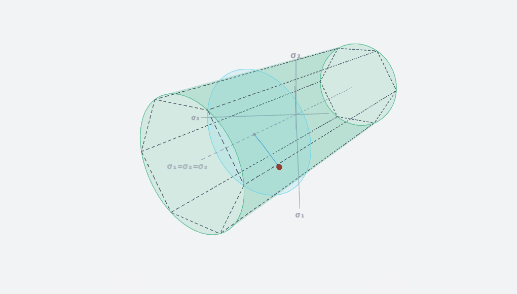
Try it yourself in the Explorer Pick the Purely hydrostatic preset. All three normal stresses are equal, no shear. Result: σv = 0, verdict elastic, no matter how large you make the values. The red sphere sits exactly on the space diagonal of the cylinder.

And this brings us back to the cube from the deep sea.

The deep-sea cube

100 MPa from all sides on a solid steel cube. That is a purely hydrostatic state: no deviator, no shape change, no yielding. Its equivalent stress is practically zero. Even at 1,000 MPa on all sides, the solid cube would not yield.

Careful, the intuition transfers wrongly to a submarine. A submarine is not a solid cube. Thin-walled hollow bodies convert external pressure into bending and shear, and those produce a real deviator. But the takeaway holds: yielding comes from shape change, not volume change. That is exactly what σv measures.

Von Mises: only the shape change

Now to make it concrete, via an intermediate step. If you rotate the imagined cube into the right position, all shear stresses disappear. Left over are three normal stresses σ₁, σ₂, σ₃, the principal stresses. Six values became three.

The von Mises equivalent stress counts only the differences of these three:

σv = √( ½ · [ (σ₁ − σ₂)² + (σ₂ − σ₃)² + (σ₃ − σ₁)² ] )

Only differences. If all three principal stresses are equal (the all-sided case), every difference is zero and σv = 0. That is why the deep-sea cube was at zero. The formal name behind this is the shape-change energy hypothesis: yielding begins when the energy of pure shape change reaches the material limit.

A useful self-check: in the uniaxial tensile test (σ₂ = σ₃ = 0), the formula gives σv = σ₁. That is exactly why you can compare σv directly with the yield strength: they are calibrated to the same scale.

Try it yourself in the Explorer Pick the Uniaxial tension preset (σx = 200, everything else zero) and leave Re at 235. The Explorer shows σv = 200, the same value as σ₁, verdict elastic, safety around 1.18. Now push σx up until the verdict flips to Yielding: at 235 MPa the yield strength is reached. For contrast, pick Pure shear: a pure shear stress alone already produces a noticeable equivalent stress (σv = √3 · τ), even though no normal stress is present.

The yield surface: a picture of the whole stress space

Up to here it was all formulas. Now the geometric picture that ties every case above together.

Spread out three axes, σ₁, σ₂, σ₃. Every stress state is then a point in this space. On the space diagonal σ₁ = σ₂ = σ₃ lie all purely hydrostatic states; no yielding occurs there. The deep-sea cube sits exactly on this line.

The von Mises condition becomes a cylinder around the diagonal in this space. The distance of your point from the axis is the shape change: inside is elastic, on the surface yielding begins. If you look along the diagonal at the cylinder, it becomes a circle. And Tresca, the shear-stress hypothesis, is the hexagon inscribed in that circle: slightly more conservative, because it never sits outside the circle.

The third hypothesis in the Explorer has a different shape. Rankine, the maximum-normal-stress hypothesis, evaluates only the largest single principal stress, independent of the other two. In principal-stress space this becomes an axis-aligned cube. The critical difference: the cylinder and hexagonal prism are open along the diagonal, the cube is closed. Rankine therefore also caps purely hydrostatic tension. That is why a purely hydrostatic state sits close to the limit under Rankine, while von Mises and Tresca give σv = 0 for the same state.

Try it yourself in the Explorer Click View along diagonal. The cylinder becomes a circle, and you can see immediately whether your point is inside it or on the edge. Toggle on Tresca, the hexagon sits cleanly inside the circle, and Rankine, which is the cube. Back in Perspective, it is clearest that the cube is bounded along the diagonal, while the cylinder and prism stay open. Rotate the view freely, enter your own six values, and watch how the red point moves.

The material chooses the hypothesis

One last point, decisive in practice: von Mises is not always the right question.

• Ductile (steel, aluminium): failure begins with yielding, that is, shape change. You compare σv per von Mises against the yield strength Re. That is the standard behind almost every contour plot. Tresca is the more conservative variant in the same family.
• Brittle (cast iron, ceramics, hardened steels): these materials barely yield, they fracture. Here you evaluate the largest principal stress σ₁ against the tensile strength Rm. This hypothesis is called Rankine.

Put shortly: von Mises answers "does it yield?" For a brittle material that is the wrong question. There the question is "does it crack?"

Try it yourself in the Explorer Stay on the Purely hydrostatic preset and toggle through the hypotheses. Von Mises and Tresca produce no yielding (σv = 0). Rankine, on the other hand, reaches its limit, because tension acts in every direction. At the same state, the hypotheses come to different verdicts. Which one applies is chosen by the material, not by habit.

Back to the colourful image

Now the contour plot reads differently. What it shows is, at every point, the full tensor, condensed into an equivalent stress so it can be compared with the data sheet.

Two things worth remembering. First: the colour is a hypothesis about yielding, not a measurement. It applies to ductile materials and ignores the hydrostatic component, deliberately. Second, and the more important point in practice: red means maximum of this scale, not automatically broken. Check the scale first, then hold σv against the yield strength.

Three sentences that should stick:

1. Six numbers, one decision. σv makes the stress tensor comparable to the tensile test.
2. Yielding comes from shape change. The hydrostatic component does not count. The deep-sea cube proves it.
3. Von Mises applies to ductile materials. For brittle materials, evaluate the largest principal stress against Rm.

Try it yourself

The fastest way to internalise all of this is to turn the dials yourself. In the Stress Space Explorer embedded below, you enter a tensor and see the principal stresses, the equivalent stress, the safety factor, and the point in space update in real time, with all three hypotheses to switch between. Take five minutes and run through the examples above.

You can also open the Explorer in a new tab if you prefer.

And that is exactly what we are aiming at with Dr.Q: simulation should not sit with a few specialists, it should be understandable and usable early in the design workflow. If you want to see how a trustworthy contour plot is generated in Dr.Q without hours of model setup, book a short online demo.

One honest note at the end: the Explorer and this article show the mechanics for illustration. They do not replace a formal strength verification.